Bengio's Neural Probabilistic Language Model (2003)

In 2003, Yoshua Bengio, Réjean Ducharme, Pascal Vincent, and Christian Jauvin published A Neural Probabilistic Language Model in the Journal of Machine Learning Research (JMLR).

Today, this paper is universally recognized as the foundational pillar of modern deep learning for natural language processing. It introduced two concepts that remain at the heart of modern Large Language Models:

1. Distributed continuous word representations (word embeddings), replacing discrete orthogonal symbols with dense vectors in $\mathbb{R}^m$.
2. Probability density estimation via neural networks, replacing combinatorial frequency counting tables with a smooth, differentiable function that generalizes across unseen combinations.

This article provides an end-to-end technical dissection of Bengio et al.’s model: the problem it solved, its mathematical formulation, its dual-path architecture, its gradient mechanics, and the computational bottlenecks that catalyzed twenty years of NLP research.

---

1. The Pre-2003 Paradigm: The Curse of Dimensionality

A language model estimates the joint probability distribution over sequences of words $W = (w_1, w_2, \dots, w_T)$ drawn from a finite vocabulary $\mathcal{V}$:

$P(W) = \prod_{t=1}^T P(w_t \mid w_1, \dots, w_{t-1}) = \prod_{t=1}^T P(w_t \mid w_{<t})$

Before Bengio’s work, language modeling was dominated by statistical n-gram models, which relied on a stationary Markov assumption of order $n-1$:

$P(w_t \mid w_{<t}) \approx P(w_t \mid w_{t-n+1}, \dots, w_{t-1}) = \frac{C(w_{t-n+1}, \dots, w_{t-1}, w_t)}{C(w_{t-n+1}, \dots, w_{t-1})}$

Where $C(\cdot)$ denotes the count of exact phrase occurrences in a training corpus.

Why Discrete Counting Collapses

Count-based statistical language modeling was crippled by two fundamental limitations:

1. Exponential State-Space Explosion

The conditioning context consists of $n-1$ tokens. The number of free parameters required to store conditional probabilities for an n-gram table is:

$|\mathcal{V}|^{n-1} \cdot (|\mathcal{V}| - 1) \sim \mathcal{O}(|\mathcal{V}|^n)$

For a modest vocabulary of $|\mathcal{V}| = 50,000$ and a modest context window of $n=5$ (4 conditioning words), the parameter space demands:

$50,000^4 \approx 6.25 \times 10^{18} \text{ values}$

Even the largest internet corpora can observe only an infinitesimally tiny fraction of these combinations. The vast majority of valid linguistic combinations never appear in the training data, leading to extreme sparsity.

2. Orthogonality and Zero Semantic Generalization

In discrete statistical models, words are symbolic atoms represented by standard basis (one-hot) vectors:

$\mathbf{v}_{\text{cat}} = [0, \dots, 0, 1, 0, \dots, 0]^\top, \quad \mathbf{v}_{\text{kitten}} = [0, \dots, 0, 0, 1, \dots, 0]^\top$

The Euclidean distance between any two distinct words is always:

$\|\mathbf{v}_i - \mathbf{v}_j\|_2 = \sqrt{2} \quad (\forall i \neq j)$

And their inner product is zero:

$\mathbf{v}_i^\top \mathbf{v}_j = 0$

Because the representation contains no notion of semantic similarity or syntactic distance, observation of:

• “The cat walked across the street”

imparts zero statistical evidence about the likelihood of:

• “The kitten walked across the street”

Traditional techniques attempted to patch this using smoothing algorithms (Jelinek-Mercer interpolation, Good-Turing discounting, and Modified Kneser-Ney). However, smoothing merely backs off to lower-order n-grams ($n-1, n-2, \dots, 1$). It redistribution rules are purely frequency-driven; it cannot share statistical strength across semantically analogous sentences.

---

2. Bengio’s Conceptual Leap: Distributed Representations

Bengio et al. proposed to solve both the curse of dimensionality and the generalization crisis simultaneously through three interrelated ideas:

1. Continuous Feature Vectors: Associate each word $i \in \mathcal{V}$ with a real-valued distributed feature vector $C(i) \in \mathbb{R}^m$, where $m \ll |\mathcal{V}|$ (typically $m \in [30, 100]$ in 2003; now $m \in [2048, 8192]$).
2. Smooth Neural Mapping: Formulate the conditional probability $P(w_t \mid w_{t-n+1}, \dots, w_{t-1})$ as a continuous, differentiable neural network function taking the concatenated feature vectors as input.
3. Simultaneous Optimization: Learn the word feature vectors $C$ and the weights of the neural probability function together using gradient descent.

The Continuous Probability Surface

Because the neural network is composed of continuous, smooth operations ($\tanh$, linear matrix multiplications, softmax), small perturbations in the input feature vectors produce small, smooth changes in the predicted output probabilities:

$C(\text{"kitten"}) \approx C(\text{"cat"}) \implies P(w_t \mid \dots, \text{"kitten"}) \approx P(w_t \mid \dots, \text{"cat"})$

If the model encounters “The cat walked across the street” during training, backpropagation adjusts the coordinates of $C(\text{"cat"})$, $C(\text{"walked"})$, and $C(\text{"street"})$. Because $C(\text{"kitten"})$ naturally clusters near $C(\text{"cat"})$ due to shared surrounding contexts elsewhere in the corpus, the model automatically assigns high probability to “The kitten walked across the street”, even if that exact sequence of words was never observed in training.

---

3. The Architecture of the Neural Language Model

Below is the complete architectural layout of Bengio’s 2003 Neural Probabilistic Language Model (NPLM):

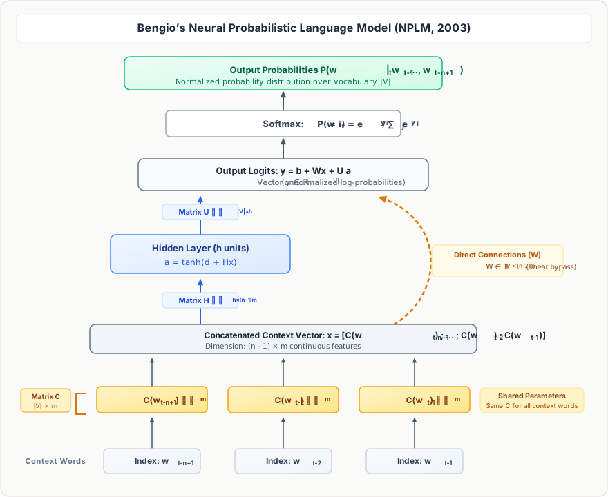
The model consists of four sequential stages: Input Lookup, Feature Concatenation, Dual-Pathway Processing, and Softmax Normalization.

3.1. Word Feature Lookup Matrix ($C$)

Let the context consist of the previous $n-1$ words:

$(w_{t-n+1}, \dots, w_{t-2}, w_{t-1})$

Each word $w \in \mathcal{V}$ is an integer index in $\{1, 2, \dots, |\mathcal{V}|\}$.

The feature lookup matrix is:

$C \in \mathbb{R}^{|\mathcal{V}| \times m}$

Where row (or column) $i$ represents the $m$-dimensional continuous distributed embedding of word $i$.

Crucial Architectural Detail: The exact same matrix $C$ is shared across all $n-1$ input positions. Whether a word appears at position $t-1$ or position $t-3$, its semantic identity is projected through the identical embedding matrix $C$.

For word $w_{t-k}$, the lookup operation extracts its embedding:

$\mathbf{e}_{t-k} = C(w_{t-k}) \in \mathbb{R}^m$

3.2. Context Concatenation ($\mathbf{x}$)

The $n-1$ extracted embedding vectors are concatenated in temporal order into a single composite context vector $\mathbf{x}$:

$\mathbf{x} = \left[ C(w_{t-n+1}) ; C(w_{t-n+2}) ; \dots ; C(w_{t-1}) \right] \in \mathbb{R}^{(n-1)m}$

The dimensionality of $\mathbf{x}$ scales linearly with context length:

$\dim(\mathbf{x}) = (n - 1) \cdot m$

3.3. Dual-Pathway Processing: Hidden Layer + Direct Connections

Bengio’s model maps the context vector $\mathbf{x}$ to unnormalized output logits $\mathbf{y} \in \mathbb{R}^{|\mathcal{V}|}$ using two parallel pathways:

Pathway 1: The Non-Linear Hidden Layer

The context vector $\mathbf{x}$ feeds into a fully connected layer with $h$ hidden units and a hyperbolic tangent ($\tanh$) activation:

$\mathbf{a} = \tanh(\mathbf{d} + H\mathbf{x})$

• $H \in \mathbb{R}^{h \times (n-1)m}$: Hidden weight matrix.
• $\mathbf{d} \in \mathbb{R}^h$: Hidden layer bias vector.
• $\mathbf{a} \in \mathbb{R}^h$: Activated hidden states.

The hidden representation is then projected to vocabulary space through matrix $U$:

$\mathbf{y}_{\text{hidden}} = U \mathbf{a} = U \tanh(\mathbf{d} + H\mathbf{x})$

• $U \in \mathbb{R}^{|\mathcal{V}| \times h}$: Output projection matrix.

Pathway 2: Direct Linear Skip Connections ($W$)

In addition to the non-linear hidden path, Bengio introduced a direct linear bypass connecting context $\mathbf{x}$ directly to output logits:

$\mathbf{y}_{\text{direct}} = W \mathbf{x}$

• $W \in \mathbb{R}^{|\mathcal{V}| \times (n-1)m}$: Direct skip connection matrix.

Why Did Bengio Include Direct Connections? The direct connection $W$ provides a linear shortcut. It allows the model to easily fit simple linear dependencies—effectively learning a smooth linear n-gram / unigram prior—leaving the hidden layer $\tanh(H\mathbf{x})$ free to dedicate its capacity to learning non-linear cross-feature interactions. (Bengio noted that setting $W = 0$ works, but keeping $W$ yields slightly faster convergence and lower perplexity).

3.4. Logits and Softmax Normalization

Combining both pathways along with an output bias vector $\mathbf{b} \in \mathbb{R}^{|\mathcal{V}|}$, the total score (logit) vector is:

$\mathbf{y} = \mathbf{b} + W \mathbf{x} + U \tanh(\mathbf{d} + H \mathbf{x})$

For each individual word $i \in \{1, \dots, |\mathcal{V}|\}$, its logit is:

$y_i = b_i + W_i \mathbf{x} + U_i \mathbf{a}$

Where $W_i$ is the $i$-th row of $W$, and $U_i$ is the $i$-th row of $U$.

Finally, the logits are normalized into a valid categorical probability distribution via the Softmax function:

$P(w_t = i \mid w_{t-n+1}, \dots, w_{t-1}) = \frac{\exp(y_i)}{\sum_{j=1}^{|\mathcal{V}|} \exp(y_j)}$

---

4. Parameter Breakdown and Dimensionality

Let us examine the total parameter inventory $\theta = \{C, H, \mathbf{d}, U, W, \mathbf{b}\}$:

Parameter	Matrix Dimensions	Description	Scale in Bengio 2003
$C$	$	\mathcal{V}	\times m$
$H$	$h \times (n-1)m$	Context-to-hidden weight matrix	Dependent on context size $n$
$\mathbf{d}$	$h \times 1$	Hidden layer bias vector	Size of hidden dimension $h$
$U$	$	\mathcal{V}	\times h$
$W$	$	\mathcal{V}	\times (n-1)m$
$\mathbf{b}$	$	\mathcal{V}	\times 1$

Total Free Parameters Formula:

$|\theta| = \underbrace{|\mathcal{V}| \cdot m}_{\text{Embeddings } C} + \underbrace{h \cdot (n-1)m + h}_{\text{Hidden layer } H, \mathbf{d}} + \underbrace{|\mathcal{V}| \cdot h}_{\text{Output } U} + \underbrace{|\mathcal{V}| \cdot (n-1)m}_{\text{Direct skip } W} + \underbrace{|\mathcal{V}|}_{\text{Output bias } \mathbf{b}}$

Factoring by vocabulary size $|\mathcal{V}|$:

$|\theta| = |\mathcal{V}| \cdot \Big( m + h + (n-1)m + 1 \Big) + h \cdot \Big( (n-1)m + 1 \Big)$

Concrete Numerical Example (From Bengio et al., 2003)

Consider typical hyperparameters from the paper:

• Vocabulary size: $|\mathcal{V}| = 17,964$
• Context order: $n = 5$ (so $n-1 = 4$ context words)
• Feature vector size: $m = 30$
• Hidden units: $h = 100$

Calculating each component:

• $C$: $17,964 \times 30 = 538,920$
• $H$: $100 \times (4 \times 30) = 100 \times 120 = 12,000$
• $\mathbf{d}$: $100$
• $U$: $17,964 \times 100 = 1,796,400$
• $W$: $17,964 \times 120 = 2,155,680$
• $\mathbf{b}$: $17,964$

$\text{Total Parameters} \approx 4,520,000 \text{ (~4.52 Million parameters)}$

Notice where the bulk of the parameter weight lies:

• The hidden layer $H$ has only 12,000 weights ($0.26\%$).
• The vocabulary-dependent matrices ($U, W, C$) account for over 99.7% of all model parameters!

Unlike count tables that explode exponentially as $\mathcal{O}(|\mathcal{V}|^n)$, Bengio’s neural model scales linearly with context length: $\mathcal{O}(n \cdot m \cdot |\mathcal{V}|)$.

---

5. Mathematical Mechanics: Loss and Backpropagation

The training objective is penalized maximum log-likelihood across a corpus of $T$ tokens:

$\mathcal{L}(\theta) = \frac{1}{T} \sum_{t=1}^T \log P(w_t \mid w_{t-n+1}, \dots, w_{t-1}) - \frac{\lambda}{2} \|\theta\|^2$

For a single training example at time $t$ where target token is $y^* = w_t$, the negative log-likelihood loss is:

$\mathcal{E} = -\log P(w_t \mid w_{<t}) = -\log \left( \frac{\exp(y_{w_t})}{\sum_{j=1}^{|\mathcal{V}|} \exp(y_j)} \right) = -y_{w_t} + \log \sum_{j=1}^{|\mathcal{V}|} \exp(y_j)$

5.1. Logit Gradients

Differentiating $\mathcal{E}$ with respect to logit $y_i$:

$\frac{\partial \mathcal{E}}{\partial y_i} = -\mathbf{1}_{\{i = w_t\}} + \frac{\exp(y_i)}{\sum_j \exp(y_j)} = P(w_t = i \mid w_{<t}) - \mathbf{1}_{\{i = w_t\}}$

Let vector $\mathbf{g}_{\mathbf{y}} = \nabla_{\mathbf{y}} \mathcal{E} \in \mathbb{R}^{|\mathcal{V}|}$. Its components are:

$g_{\mathbf{y}, i} = P(w_t = i) - \delta_{i, w_t}$

Where $\delta_{i, w_t}$ is the Kronecker delta. The error signal is simply the predicted probability minus the true one-hot target.

5.2. Gradients for Output Weights and Hidden Units

Applying the chain rule:

$\frac{\partial \mathcal{E}}{\partial U} = \mathbf{g}_{\mathbf{y}} \mathbf{a}^\top \in \mathbb{R}^{|\mathcal{V}| \times h}$

$\frac{\partial \mathcal{E}}{\partial W} = \mathbf{g}_{\mathbf{y}} \mathbf{x}^\top \in \mathbb{R}^{|\mathcal{V}| \times (n-1)m}$

$\frac{\partial \mathcal{E}}{\partial \mathbf{b}} = \mathbf{g}_{\mathbf{y}} \in \mathbb{R}^{|\mathcal{V}|}$

The gradient propagating back into the hidden activation vector $\mathbf{a}$:

$\mathbf{g}_{\mathbf{a}} = \frac{\partial \mathcal{E}}{\partial \mathbf{a}} = U^\top \mathbf{g}_{\mathbf{y}} \in \mathbb{R}^h$

Passing through the non-linear hyperbolic tangent activation $\mathbf{a} = \tanh(\mathbf{z})$ where $\mathbf{z} = \mathbf{d} + H\mathbf{x}$:

$\mathbf{g}_{\mathbf{z}} = \mathbf{g}_{\mathbf{a}} \odot (1 - \mathbf{a}^2) \in \mathbb{R}^h$

$\frac{\partial \mathcal{E}}{\partial H} = \mathbf{g}_{\mathbf{z}} \mathbf{x}^\top \in \mathbb{R}^{h \times (n-1)m}, \quad \frac{\partial \mathcal{E}}{\partial \mathbf{d}} = \mathbf{g}_{\mathbf{z}} \in \mathbb{R}^h$

5.3. Backpropagation into the Context Vector $\mathbf{x}$

Both the direct connection $W$ and the hidden layer $H$ contribute to the gradient of the concatenated input vector $\mathbf{x}$:

$\mathbf{g}_{\mathbf{x}} = \frac{\partial \mathcal{E}}{\partial \mathbf{x}} = W^\top \mathbf{g}_{\mathbf{y}} + H^\top \mathbf{g}_{\mathbf{z}} \in \mathbb{R}^{(n-1)m}$

5.4. Updating the Word Embedding Matrix $C$

Because $\mathbf{x}$ is the concatenation of $n-1$ feature vectors:

$\mathbf{x} = [\mathbf{e}_{t-n+1} ; \dots ; \mathbf{e}_{t-1}]$

We slice $\mathbf{g}_{\mathbf{x}}$ into $n-1$ chunks of dimension $m$:

$\frac{\partial \mathcal{E}}{\partial C(w_{t-k})} = \mathbf{g}_{\mathbf{x}}[(k-1)m : km] \in \mathbb{R}^m \quad \text{for } k \in \{1, \dots, n-1\}$

Sparse Gradient Updates: In a vocabulary of 50,000 words, only the $n-1$ word vectors present in the current context receive non-zero gradient updates at step $t$: $C(w_{t-k}) \leftarrow C(w_{t-k}) - \eta \left( \frac{\partial \mathcal{E}}{\partial C(w_{t-k})} + \lambda C(w_{t-k}) \right)$ All other rows in $C$ remain untouched during this step.

---

6. The Computational Bottleneck: The Output Softmax

While Bengio’s NPLM conquered the curse of dimensionality, it ran directly into a severe computational barrier: the cost of computing the denominator in the softmax function.

$P(w_t = i) = \frac{\exp(y_i)}{\sum_{j=1}^{|\mathcal{V}|} \exp(y_j)}$

To perform a single parameter update at step $t$:

1. The model must compute the logit $y_j$ for every single word $j$ in the entire vocabulary $\mathcal{V}$.
2. This requires the full matrix-vector product $U \mathbf{a}$ and $W \mathbf{x}$, which costs:

$\mathcal{O}(|\mathcal{V}| \cdot h + |\mathcal{V}| \cdot (n-1)m) \text{ floating point operations per token}$

In 2003, modern GPUs did not exist for machine learning. Training Bengio’s model with $|\mathcal{V}| \approx 18,000$ on 14 million words took 3 weeks on a cluster of 40 CPUs running parallelized asynchronous stochastic gradient descent.

                      The 2003 Softmax Bottleneck:
                      
   Hidden state a (h = 100)
             │
             ▼
   Matrix Multiply: U ∈ ℝ^{|V| × h}   ◄── Computing scores for ALL 18,000+ words
             │                            at EVERY training step!
             ▼
   Unnormalized Logits y ∈ ℝ^{|V|}
             │
             ▼
   Denominator Sum: ∑_{j=1}^{|V|} exp(y_j)

The Inventions Spawned by this Bottleneck

This exact bottleneck stimulated a decade of groundbreaking machine learning research to approximate or accelerate the softmax:

1. Hierarchical Softmax (Morin & Bengio, 2005; Mnih & Hinton, 2009): Organized the vocabulary into a balanced binary tree or WordNet hierarchy. Evaluating word probability required only walking from root to leaf, reducing complexity from $\mathcal{O}(|\mathcal{V}|)$ to $\mathcal{O}(\log_2 |\mathcal{V}|)$.
2. Importance Sampling & NCE (Noise-Contrastive Estimation, Gutmann & Hyvärinen, 2010; Mnih & Teh, 2012): Transformed the multi-class density estimation problem into binary classification (discriminating real target tokens from noise samples).
3. Negative Sampling in Word2Vec (Mikolov et al., 2013): Simplified NCE by sampling only $k \approx 5\text{–}20$ negative tokens per target word, completely bypassing the $|\mathcal{V}|$ denominator and allowing Word2Vec to train on billions of tokens in hours on a single desktop.

---

7. Experimental Results: Does It Actually Work?

Bengio et al. tested their model on two standard benchmarks of the time:

• Brown Corpus: 1,181,041 words; vocabulary pruned to $|\mathcal{V}| = 16,383$.
• Associated Press (AP) News: 14 million words; vocabulary pruned to $|\mathcal{V}| = 17,964$.

Evaluation was performed using Perplexity (PPL), which measures the inverse geometric mean probability assigned to the test tokens:

$\text{PPL} = \exp\left( -\frac{1}{T_{\text{test}}} \sum_{t=1}^{T_{\text{test}}} \log P(w_t \mid w_{<t}) \right)$

Lower perplexity indicates a superior, more confident predictive model.

Key Results on AP News (Validation Perplexity)

Model Architecture	Context Size ($n$)	Validation Perplexity	Relative Improvement
Smoothed Trigram (Kneser-Ney)	$n=3$	125.2	Baseline
Smoothed 4-gram (Kneser-Ney)	$n=4$	123.0	$-1.7\%$
Smoothed 5-gram (Kneser-Ney)	$n=5$	121.5	$-3.0\%$
Bengio Neural LM (MLP alone)	$n=5$ ($m=60, h=100$)	113.2	$-9.6\%$
Bengio Neural LM (Interpolated with N-gram)	$n=5$	109.4	$-12.6\%$

Critical Findings from the Paper:

1. Dramatic Perplexity Drop: The neural language model achieved a roughly 10% to 20% relative perplexity reduction over state-of-the-art interpolated and Kneser-Ney smoothed n-grams.
2. Model Ensembling / Interpolation: Bengio discovered that interpolating the predictions of the neural model with an n-gram model: $P_{\text{ensemble}}(w_t) = \alpha P_{\text{neural}}(w_t) + (1-\alpha) P_{\text{n-gram}}(w_t)$ outperformed either model alone. The n-gram was effective at memorizing frequent local idiomatic bigrams/trigrams, while the neural network generalized across broad semantic contexts.
3. Emergence of Semantic Vector Spaces: When Bengio visualized the 30-dimensional learned word representations $C(w)$ using 2D projections, the vectors naturally formed semantic clusters:
   • Grammatical parts of speech grouped together (determiners with determiners, verbs with verbs).
   • Synonyms and co-hyponyms (“cat”, “dog”, “rabbit”) mapped to adjacent coordinates in the vector space.

---

8. Bengio’s Model vs. The Modern Transformer

How does Bengio’s 2003 formulation compare to modern Large Language Models like GPT-4 or LLaMA?

Dimension	Bengio NPLM (2003)	Modern Decoder Transformer (e.g. GPT / LLaMA)
Word Representation	Matrix $C \in \mathbb{R}^{	\mathcal{V}
Context Aggregation	Fixed-length vector concatenation: $\mathbf{x} = [C(w_{t-n+1}) ; \dots ; C(w_{t-1})]$	Causal Multi-Head Self-Attention: $A = \text{softmax}\left(\frac{QK^\top}{\sqrt{d_k}} + M\right)V$
Context Length ($n$)	Fixed window of $4\text{–}5$ words	Dynamic sequence of $4,000$ to $1,000,000+$ tokens
Non-Linear Transform	Single shallow hidden layer: $\tanh(d + H\mathbf{x})$	Deep stacked Transformer blocks ($32\text{–}128$ layers) with SwiGLU / GeLU MLPs
Output Head	Logits $\mathbf{y} = b + W\mathbf{x} + U\mathbf{a}$	Linear head with tied or untied weights: $\mathbf{y} = W_{\text{unembed}} \text{LayerNorm}(\mathbf{h}_L)$
Probability Function	Softmax over vocabulary $	\mathcal{V}
Optimization	Maximizing log-likelihood via SGD	Maximizing log-likelihood via AdamW + FP8/BF16 mixed precision

What Changed?

1. From Concatenation to Self-Attention: Bengio’s concatenation assumed a rigid context size ($n-1$). A token at position $t-1$ occupied fixed dimensions $[0:m]$ in $\mathbf{x}$, while a token at $t-2$ occupied $[m:2m]$. There was no position-invariant relational reasoning. Self-attention replaced concatenation with content-based pairwise routing.
2. From Words to Subwords: Bengio used full dictionary words, leading to large out-of-vocabulary (OOV) issues or huge matrices. Modern LLMs use subword tokenization (Byte-Pair Encoding, WordPiece), fixing $|\mathcal{V}|$ typically between 32,000 and 128,000 while maintaining open-vocabulary coverage.
3. Depth: Bengio’s model was 2 layers deep (embedding $\to$ hidden $\to$ output). Modern LLMs stack dozens of Transformer layers with residual connections and RMSNorm.

What Remained Identical?

The macro-objective is fundamentally unchanged:

• Every token is mapped to a continuous vector via an embedding table.
• A parameterized network computes logits across the vocabulary.
• The model is trained via self-supervised autoregressive next-token prediction using cross-entropy loss over a Softmax distribution.

---

9. Summary & Enduring Legacy

Yoshua Bengio’s 2003 paper accomplished three historic feats:

1. Proved the viability of distributed representations for language: It validated the connectionist hypothesis (Hinton, 1986) on real-world, large-scale linguistic data.
2. Broke the curse of dimensionality: By treating probability estimation as a continuous regression problem rather than discrete combinatorial counting, it introduced semantic generalization to machine learning.
3. Laid the foundational template for all modern generative models: Every neural architecture that followed—Word2Vec, LSTMs, BERT, and GPT—is an evolution of the distributed probabilistic paradigm introduced in this landmark paper.

---

References

1. Bengio, Y., Ducharme, R., Vincent, P., & Jauvin, C. (2003). A Neural Probabilistic Language Model. Journal of Machine Learning Research (JMLR), 3(Feb), 1137-1155.
2. Hinton, G. E. (1986). Learning distributed representations of concepts. Proceedings of the eighth annual conference of the cognitive science society, 1, 1-12.
3. Morin, F., & Bengio, Y. (2005). Hierarchical Probabilistic Neural Network Language Model. AISTATS.
4. Mikolov, T., Chen, K., Corrado, G., & Dean, J. (2013). Efficient Estimation of Word Representations in Vector Space. arXiv:1301.3781.
5. Vaswani, A., et al. (2017). Attention Is All You Need. Advances in Neural Information Processing Systems (NeurIPS).