Neural Network Learning - 1. From Linear to Nonlinear

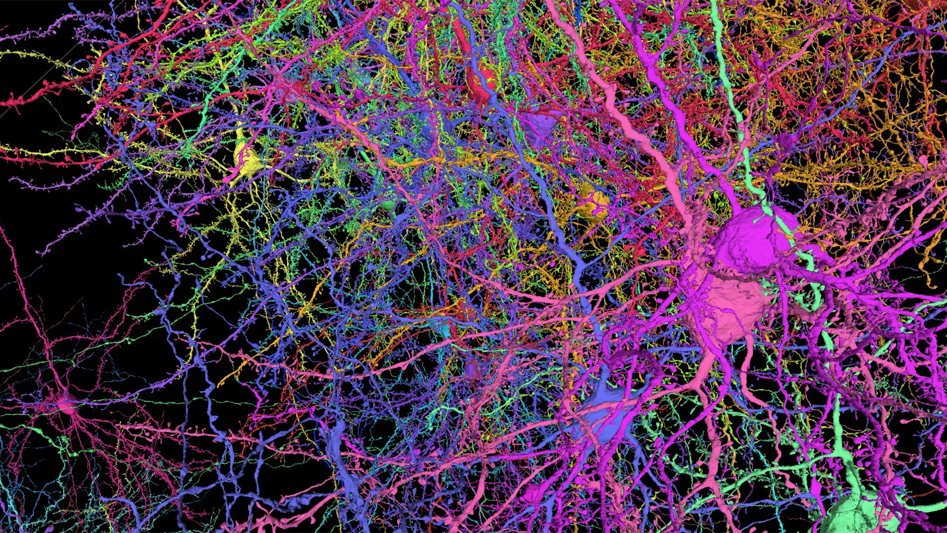
A neural network is actually very simple:

A Neuron:

$z=w_1x_1+w_2x_2+\cdots+w_nx_n+b$

The activation function:

$a=\sigma(z)$

But this neuron is not a biological neuron—it is merely inspired by the brain. A neuron receives multiple inputs (X) and finally outputs a weighted sum.

W is like the axon of a biological neuron, computing over all the input neurons one by one.

Turing: Can Machines Think?

The human brain is made up of tens of billions of neurons, connected to each other through synapses, transmitting information via electrical and chemical signals. When a neuron receives stimulation from other neurons, a change in potential builds up inside the cell; when this change reaches a certain threshold, the neuron is activated and passes the signal on to the next neuron.

Why does material neural activity give rise to thought, feeling, and self-awareness?

Why can a system made of matter turn around and come to know the world—even to know itself?

From microscopic neural activity to macroscopic thought and consciousness, there seems to span a gap that has yet to be fully explained.

In 1950, the British mathematician Alan Turing published his famous paper, Computing Machinery and Intelligence.

At the beginning of this paper, he posed a question that would later become extremely famous:

$$\text{Can machines think?}$$

Turing did not try to directly define “thinking” or “intelligence.” These concepts are too abstract and too easily mired in philosophical debate.

Instead, he took a more practical approach: if a machine behaves indistinguishably from a human in conversation, can we then consider it to possess some kind of intelligence?

This idea later became known as the Turing Test.

Turing’s truly important contribution to artificial intelligence is not that he gave a final definition of intelligence, but that he turned “whether machines can think” into a question that can be discussed, tested, and engineered.

The MP Neuron Model

Can complex intelligence emerge from the collective behavior of simple computational units?

In 1943, Warren McCulloch and Walter Pitts proposed an early mathematical model of an artificial neuron, later commonly known as the MP neuron model.

The model is very simple: it receives multiple inputs, sums them up, and then decides whether to output 1 through a simple threshold check.

It receives multiple inputs:

$$x_1, x_2, x_3, \dots, x_n$$

In the simplest MP neuron, each input usually has only two states:

$$x_i \in {0, 1}$$

The neuron sums all its inputs and compares the result against a threshold.

If the sum reaches the threshold, it outputs 1; otherwise, it outputs 0.

$$y = \begin{cases} 1, & \sum_{i=1}^{n} x_i \geq \theta \ 0, & \sum_{i=1}^{n} x_i < \theta \end{cases}$$

If the total stimulation exceeds the threshold, the neuron is activated; if it does not exceed the threshold, the neuron is not activated.

The MP neuron can represent certain logical operations, such as AND, OR, and NOT.

But the MP neuron has no learning ability.

The Perceptron

In 1958, Frank Rosenblatt proposed the Perceptron.

The perceptron can be seen as an upgraded MP neuron. It still receives multiple inputs, but each input now has a weight associated with it.

The inputs of the perceptron can be written as:

$$x = (x_1, x_2, x_3, \dots, x_n)$$

The weights can be written as:

$$w = (w_1, w_2, w_3, \dots, w_n)$$

The perceptron first computes the weighted sum of its inputs:

$$z = w_1x_1 + w_2x_2 + w_3x_3 + \dots + w_nx_n + b$$

It can also be written in vector form:

$$z = w \cdot x + b$$

where:

$$w \cdot x = \sum_{i=1}^{n} w_i x_i$$

The bias b can be understood as a parameter that adjusts how easily the neuron is activated. If the bias is large, the neuron is easier to activate; if the bias is small, the neuron is harder to activate.

The output of the perceptron can be written as:

$$y = \begin{cases} 1, & w \cdot x + b \geq 0 \ 0, & w \cdot x + b < 0 \end{cases}$$

[COMMON] A step function is used here, which can also be written as:

$$y = f(w \cdot x + b)$$

where:

$$f(z) = \begin{cases} 1, & z \geq 0 \ 0, & z < 0 \end{cases}$$

The Geometric Meaning of the Perceptron

Essentially, the perceptron is looking for a classification boundary.

For two-dimensional input:

$$x = (x_1, x_2)$$

The perceptron’s decision condition is:

$$w_1x_1 + w_2x_2 + b = 0$$

which fits a straight line.

More generally, in high-dimensional space:

$$w \cdot x + b = 0$$

represents a hyperplane.

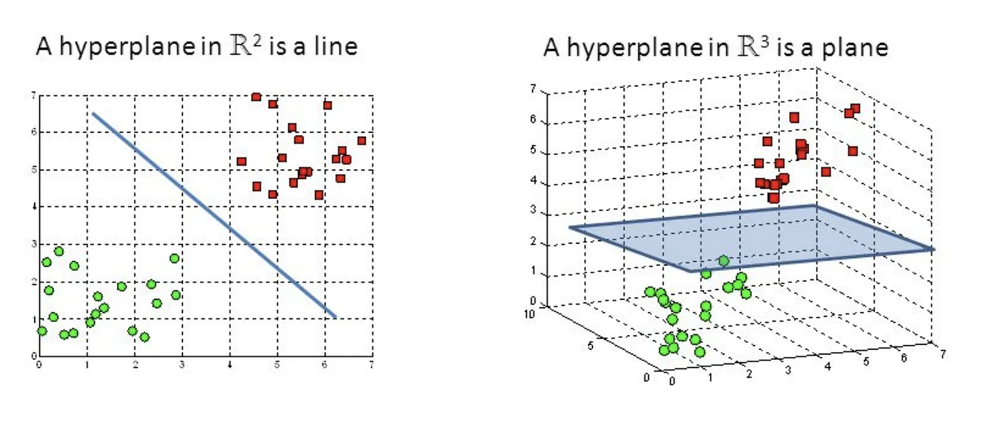
The problems a perceptron can solve are essentially classification problems that can be separated by a line, a plane, or a high-dimensional hyperplane.

The Limitations of the Perceptron

A single-layer perceptron can only solve linearly separable problems.

But many real-world problems are not linearly separable. The simplest classic example, XOR, is not linearly separable.

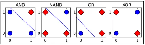
The inputs and outputs of XOR are:

$$(0,0) \rightarrow 0$$ $$(1,0) \rightarrow 1$$ $$(0,1) \rightarrow 1$$ $$(1,1) \rightarrow 0$$

Although a single-layer perceptron can learn some simple classification boundaries, it cannot express more complex nonlinear relationships.

In 1969, Marvin Minsky and Seymour Papert systematically analyzed the limits of the perceptron in their book, Perceptrons.

But the story did not really end there. If a single-layer perceptron cannot solve nonlinear problems, a natural idea arises: why not stack multiple neurons into a multilayer network?

Multilayer Perceptron (MLP)

| From Linear to Nonlinear

The key to breaking through is not abandoning neurons, but connecting them into a multilayer structure. The first layer of neurons extracts intermediate features, and the later neurons make decisions based on those features. In this way, the network can no longer only draw a straight line, but can compose more complex decision boundaries.

But without an activation function, each layer is just a linear transformation:

$$a^{(1)} = W^{(1)}x + b^{(1)}$$ $$a^{(2)} = W^{(2)}a^{(1)} + b^{(2)}$$

Substituting the first layer into the second gives:

$$a^{(2)} = W^{(2)}(W^{(1)}x + b^{(1)}) + b^{(2)}$$

Expanding:

$$a^{(2)}=W^{(2)}W^{(1)}x+W^{(2)}b^{(1)}+b^{(2)}$$

which is equivalent to:

$$a^{(2)} = W'x + b'$$

After stacking, multiple linear transformations are still essentially just one linear transformation.

Nonlinear activation functions break this limitation. They allow the network to express curved, piecewise, and complex functional relationships, rather than only drawing a line, a plane, or a hyperplane.

Activation Functions

Step Function

In early perceptrons, neurons used the step function:

$$f(z)= \begin{cases} 1, & z \geq 0 \ 0, & z < 0 \end{cases}$$

where:

$$z = w \cdot x + b$$

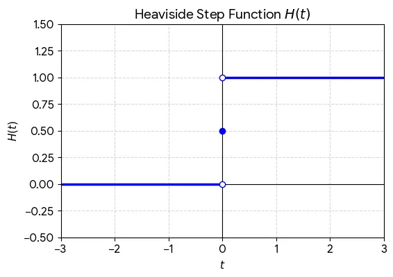
The step function is intuitive: if the input signal is strong enough, the neuron outputs 1; if it is not strong enough, the neuron outputs 0—making a binary decision.

Sigmoid

The Sigmoid function can be written as:

$$\sigma(z)=\frac{1}{1+e^{-z}}$$

[COMMON] It compresses any real number to between 0 and 1:

$$0 < \sigma(z) < 1$$

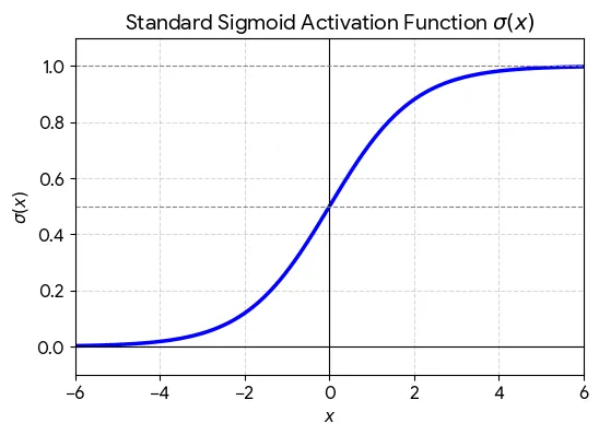
[INFERRED] This makes it well-suited for representing a “sense of probability” or “degree of activation.” [COMMON] But when the input is very large or very small, Sigmoid’s gradient becomes very small. [INFERRED] This slows down training in deep networks—the so-called vanishing gradient problem.

Tanh

The Tanh function can be written as:

$$\tanh(z)=\frac{e^z-e^{-z}}{e^z+e^{-z}}$$

[COMMON] It compresses the input to between -1 and 1:

$$-1 < \tanh(z) < 1$$

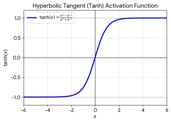
[INFERRED] Compared to Sigmoid, Tanh’s output is centered at 0, making it easier to optimize in some scenarios. [COMMON] But it can also suffer from diminishing gradients when the absolute value of the input is large.

ReLU

The ReLU function can be written as:

$$\text{ReLU}(z)=\max(0,z)$$

that is:

$$\text{ReLU}(z)= \begin{cases} z, & z > 0 \ 0, & z \leq 0 \end{cases}$$

[INFERRED] ReLU’s idea is very simple: if the input is positive, keep it; if it is negative, turn it into 0. [COMMON] ReLU is computationally simple, with stable gradients in the positive region. [KNOWN] In modern deep neural networks, ReLU and its variants are widely used. [INFERRED] Its importance lies not only in its “simple functional form,” but in that it makes deep networks easier to train.

Forward Propagation

｜ Forward Propagation: How Information Flows Layer by Layer

[COMMON] With weights, biases, and activation functions, a neuron is no longer just a simple switch, but a unit capable of continuous computation.

[COMMON] For the $l$-th layer, forward propagation can be written as:

$$z^{(l)} = W^{(l)}a^{(l-1)} + b^{(l)}$$ $$a^{(l)} = f(z^{(l)})$$

[COMMON] Here, $a^{(l-1)}$ is the previous layer’s output, $W^{(l)}$ is the current layer’s weight matrix, $b^{(l)}$ is the current layer’s bias, $f$ is the activation function, and $a^{(l)}$ is the current layer’s output.

[INFERRED] That is, each layer first performs a linear transformation on the information from the previous layer, then adds nonlinearity through the activation function, and finally passes the result on to the next layer.

[INFERRED] This process can be understood as: the previous layer passes information to the next layer, which first combines the information via weighted sums, and then decides through the activation function which information should continue to be passed on.

[COMMON] If the network has multiple layers, this process repeats:

$$x \rightarrow a^{(1)} \rightarrow a^{(2)} \rightarrow \cdots \rightarrow \hat{y}$$

[INFERRED] This is what is called forward propagation. It is like an information flow from input to output: data enters at the input layer, is continuously transformed through the hidden layers, and finally produces a prediction at the output layer.

Loss Functions

[COMMON] Forward propagation only tells us the model’s prediction, not how good that prediction is.

[COMMON] To measure the gap between the predicted value and the true value, we need a loss function.

[COMMON] Suppose the model’s predicted value is:

$$\hat{y}$$

and the true label is:

$$y$$

[COMMON] For regression problems, a common loss function is the Mean Squared Error (MSE):

$$L = \frac{1}{2}(\hat{y}-y)^2$$

[INFERRED] The larger the loss, the worse the model’s prediction; the smaller the loss, the closer the model’s prediction is to the true answer.

Gradient Descent

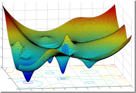
The gradient of the loss function with respect to all parameters can be written as a vector:

$$\nabla L = \left( \frac{\partial L}{\partial w_1}, \frac{\partial L}{\partial w_2}, \cdots, \frac{\partial L}{\partial b} \right)$$

Each entry in this vector is the partial derivative of the loss function with respect to one parameter.

The parameter update rule for gradient descent is:

$$\theta \leftarrow \theta - \eta \frac{\partial L}{\partial \theta}$$

where: $\theta$ denotes the model parameters, $L$ denotes the loss function, and $\eta$ denotes the learning rate.

$$\theta = {W^{(1)}, b^{(1)}, W^{(2)}, b^{(2)}, \dots, W^{(L)}, b^{(L)}}$$

The gradient tells us: when a parameter $(\theta)$ changes slightly, in which direction the loss function $(L)$ changes, and how quickly.

If the gradient is positive, moving the parameter in the increasing direction makes the loss larger.

If the gradient is negative, moving the parameter in the increasing direction makes the loss smaller.

Good Learning Resources

• http://neuralnetworksanddeeplearning.com/chap1.html
• https://www.bilibili.com/video/BV18m411S79t